The active inference framework is an approach to explaining many aspects of cognition. At its heart are two mathematical terms: free energy \(F\) and expected free energy \(G\).
Confusingly, expected free energy is not just an expectation over free energy. Its definition is slightly more involved. In previous posts I have given an intuitive description of free energy and described how it can be employed by a cognitive system. In this post I will attempt an intuitive explanation of expected free energy.
Basics
For inference and learning we use free energy. Start with a generative model over hidden states \(\class{mj_blue}{w}\) and observations \(\class{mj_red}{x}\):
$$ p(\class{mj_blue}{w},\class{mj_red}{x}) = p(\class{mj_red}{x}|\class{mj_blue}{w})p(\class{mj_blue}{w}) $$
Free energy is a function of three things: the model \(p\), an observation \(\class{mj_red}{x}\), and a set of beliefs about hidden states \(\class{mj_yellow}{q(\class{mj_blue}{w})}\):
$$ F(p,\class{mj_yellow}{q},\class{mj_red}{x}) = \sum_{\class{mj_blue}{w}} \class{mj_yellow}{q(\class{mj_blue}{w})} \log \left( \frac{\class{mj_yellow}{q(\class{mj_blue}{w})}} {p(\class{mj_blue}{w},\class{mj_red}{x})} \right) $$
The idea is to make an observation and then choose your beliefs, \(\class{mj_yellow}{q(\class{mj_blue}{w})}\), to make \(F\) as small as possible.
For action planning we use expected free energy. Expected free energy extends free energy in two ways. First, we condition our beliefs about future states on our actions \(\class{mj_green}{\pi}\):
$$ \class{mj_yellow}{q(\class{mj_blue}{w})} \rightarrow \class{mj_yellow}{q(\class{mj_blue}{w}|\class{mj_green}{\pi})} $$
Second, instead of measuring the log ratio for a single observation \(\class{mj_red}{x}\), we take the expected value over future observations:
$$ \log{\left( \frac{\class{mj_yellow}{q(\class{mj_blue}{w})}} {p(\class{mj_blue}{w},\class{mj_red}{x})} \right)} \rightarrow \sum_{\class{mj_red}{x}} p(\class{mj_red}{x}|\class{mj_blue}{w}) \log{\left( \frac{\class{mj_yellow}{q(\class{mj_blue}{w}|\class{mj_green}{\pi})}} {p(\class{mj_blue}{w},\class{mj_red}{x})} \right)} $$
The result is a function over \(p\), \(\class{mj_yellow}{q}\) and \(\class{mj_green}{\pi}\):
$$ G(p,\class{mj_yellow}{q},\class{mj_green}{\pi}) = \sum_{\class{mj_blue}{w}} \class{mj_yellow}{q(\class{mj_blue}{w}|\class{mj_green}{\pi})} \sum_{\class{mj_red}{x}} p(\class{mj_red}{x}|\class{mj_blue}{w}) \log{\left( \frac{\class{mj_yellow}{q(\class{mj_blue}{w}|\class{mj_green}{\pi})}} {p(\class{mj_blue}{w},\class{mj_red}{x})} \right)} $$
The idea is to choose your actions, \(\class{mj_green}{\pi}\), to make \(G\) as small as possible.
\(F\) and \(G\) defined (compact form)
To make the comparison between the two definitions as clear as possible:
$$ \begin{alignat}{3} F(p,\class{mj_yellow}{q},\class{mj_red}{x}) &= \sum_{\class{mj_blue}{w}} \class{mj_yellow}{q(\class{mj_blue}{w})} &&. &&\log \left( \frac{\class{mj_yellow}{q(\class{mj_blue}{w})}} {p(\class{mj_blue}{w},\class{mj_red}{x})} \right)\\[2ex] G(p,\class{mj_yellow}{q},\class{mj_green}{\pi}) &= \sum_{\class{mj_blue}{w}} \class{mj_yellow}{q(\class{mj_blue}{w}|\class{mj_green}{\pi})} \ &&. \sum_{\class{mj_red}{x}} p(\class{mj_red}{x}|\class{mj_blue}{w}) &&\log{\left( \frac{\class{mj_yellow}{q(\class{mj_blue}{w}|\class{mj_green}{\pi})}} {p(\class{mj_blue}{w},\class{mj_red}{x})} \right)} \end{alignat} $$
Three points to bear in mind:
- In \(F\), the variable \(\class{mj_red}{x}\) refers to a single observation that the agent has just seen.
- In \(G\), the variable \(\class{mj_red}{x}\) ranges over possible future observations.
- More sophisticated versions of \(G\) define different variables \(\class{mj_red}{x_t}\) for each future timestep \(t.\) For simplicity, we are assuming \(G\) is calculated for the next timestep only.
\(F\) and \(G\) make trade-offs explicit
Free energy offers a way to trade the cost of complexity for the cost of inaccuracy:
$$ F= \underbrace{ \sum_{\class{mj_blue}{w}} \left( \class{mj_yellow}{q(\class{mj_blue}{w})} \log \left( \frac{\class{mj_yellow}{q(\class{mj_blue}{w})}} {p(\class{mj_blue}{w})} \right) \right)}_{ \substack{ \text{Cost of complexity} } } \quad + \quad \underbrace{ \sum_{\class{mj_blue}{w}} \left( \class{mj_yellow}{q(\class{mj_blue}{w})} \log \left( \frac{1} {p(\class{mj_red}{x}|\class{mj_blue}{w})} \right) \right)}_{ \substack{ \text{Cost of inaccuracy} } } $$
Expected free energy offers a way to trade the cost of not satisfying your preferences for the cost of being surprised in future:
$$ G= \underbrace{ \sum_{\class{mj_blue}{w}} \left( \class{mj_yellow}{q(\class{mj_blue}{w}|\class{mj_green}{\pi})} \log \left( \frac{\class{mj_yellow}{q(\class{mj_blue}{w}|\class{mj_green}{\pi})}} {p(\class{mj_blue}{w})} \right) \right)}_{ \substack{ \text{Cost of failing to}\\ \text{satisfy your preferences} } } \quad + \quad \underbrace{ \sum_{\class{mj_blue}{w}} \left( \class{mj_yellow}{q(\class{mj_blue}{w}|\class{mj_green}{\pi})} \sum_{\class{mj_red}{x}}p(\class{mj_red}{x}|\class{mj_blue}{w}) \log \left( \frac{1} {p(\class{mj_red}{x}|\class{mj_blue}{w})} \right) \right)}_{ \substack{ \text{Cost of being}\\ \text{surprised in future} } } $$
In each case, the relevant free energy term puts the cost of each activity into a common currency. The agent can then directly compare each cost, allowing it to select the uniquely correct belief state \(\class{mj_yellow}{q}\) (for free energy) or action sequence \(\class{mj_green}{\pi}\) (for expected free energy).
There are at least two open questions here:
-
Given an unrestricted choice of \(\class{mj_yellow}{q}\), the uniquely correct value that minimises \(F\) is the true posterior \(\class{mj_yellow}{q(\class{mj_blue}{w})}=p(\class{mj_blue}{w}|\class{mj_red}{x}).\) What is the equivalent uniquely correct action sequence \(\class{mj_green}{\pi}?\) Does it correspond to an existing result, just as \(\class{mj_yellow}{q(\class{mj_blue}{w})}=p(\class{mj_blue}{w}|\class{mj_red}{x})\) corresponds to Bayes’ theorem for inference?
-
Advocates of the free energy principle make much of the fact that \(p(\class{mj_blue}{w})\) can sometimes be interpreted as the agent’s preferences. That’s what enables the interpretation of the first term of \(G\) as a measure of how far expected future states diverge from preferred states – in other words, a measure of the cost of failing to satisfy preferences. But the standard interpretation of the second term treats \(p\) as a regular probability distribution again. It’s one thing to claim that a distribution can represent preferences; it’s quite another to claim that one and the same distribution can represent both preferences and probabilities in the same equation. What legitimises this double character?
A possible answer to the second question comes from communication theory. There, \(p(x)\) is the probability of outcome \(x\) and \(\log{\frac{1}{p(x)}}\) is a measure of the cost of representing that \(x\) occurred (assuming you are using the optimal code for representing outcomes). So perhaps proponents of active inference are justified as long as they restrict themselves to interpreting \(p\) as a preference only when it appears inside a logarithm.
When \(\class{mj_green}{\pi}\) satisfies preferences
Because \(p\) is treated as representing preferences, one of the goals of action is to make \(\class{mj_yellow}{q(\class{mj_blue}{w}|\class{mj_green}{\pi})}\) match \(p(\class{mj_blue}{w}).\) Something interesting happens when this is achieved. The first term disappears because \(\log{\frac{p(\class{mj_blue}{w})}{p(\class{mj_blue}{w})}}=\log{1}=0.\) The second term becomes:
$$ \sum_{\class{mj_blue}{w}} p(\class{mj_blue}{w}) \sum_{\class{mj_red}{x}}p(\class{mj_red}{x}|\class{mj_blue}{w}) \log \left( \frac{1} {p(\class{mj_red}{x}|\class{mj_blue}{w})} \right) $$
This is the definition of conditional entropy \(H(\class{mj_red}{X}|\class{mj_blue}{W}).\)
Another face of \(G\): informational form
Expected free energy is sometimes characterised as a trade-off between epistemic goals and pragmatic goals. To see how this works, we have to rearrange \(G\) again.
$$ G= \underbrace{ \sum_{\class{mj_blue}{w}} \class{mj_yellow}{q(\class{mj_blue}{w}|\class{mj_green}{\pi})} \sum_{\class{mj_red}{x}} p(\class{mj_red}{x}|\class{mj_blue}{w}) \log{\left( \frac{\class{mj_yellow}{q(\class{mj_blue}{w}|\class{mj_green}{\pi})}} {p(\class{mj_blue}{w}|\class{mj_red}{x})} \right)} }_{ \text{Epistemic penalty} } + \underbrace{ \sum_{\class{mj_blue}{w}} \class{mj_yellow}{q(\class{mj_blue}{w}|\class{mj_green}{\pi})} \sum_{\class{mj_red}{x}} p(\class{mj_red}{x}|\class{mj_blue}{w}) \log{\left( \frac{1} {p(\class{mj_red}{x})} \right)} }_{ \text{Pragmatic penalty} } $$
Notice that here we have split \(p(\class{mj_blue}{w},\class{mj_red}{x})\) into \(p(\class{mj_blue}{w}|\class{mj_red}{x})\) and \(p(\class{mj_red}{x}).\) The previous form resulted from splitting it into \(p(\class{mj_red}{x}|\class{mj_blue}{w})\) and \(p(\class{mj_blue}{w}).\) Deriving these two different forms from these two different splits is exactly how we derive the two different forms of \(F\).
Nevertheless, the resulting equation for \(G\) is pretty ugly! But something magical happens when you let \(\class{mj_yellow}{q(\class{mj_blue}{w}|\class{mj_green}{\pi})} = p(\class{mj_blue}{w}):\)
$$ G= \sum_{\class{mj_blue}{w},\class{mj_red}{x}} p(\class{mj_blue}{w},\class{mj_red}{x}) \log{\left( \frac{p(\class{mj_blue}{w})} {p(\class{mj_blue}{w}|\class{mj_red}{x})} \right)} + \sum_{\class{mj_blue}{w},\class{mj_red}{x}} p(\class{mj_blue}{w},\class{mj_red}{x}) \log{\left( \frac{1} {p(\class{mj_red}{x})} \right)} $$
I know what you’re thinking: “That doesn’t look very magical!” Well, you’re only a little bit wrong. The first term is the negative of the mutual information between hidden states and observations:
$$ G= -I(\class{mj_blue}{W};\class{mj_red}{X})+ \sum_{\class{mj_blue}{w},\class{mj_red}{x}} p(\class{mj_blue}{w},\class{mj_red}{x}) \log{\left( \frac{1} {p(\class{mj_red}{x})} \right)} $$
while the second term is an unusual way of writing the entropy of observations:
$$ G= -I(\class{mj_blue}{W};\class{mj_red}{X})+ H(\class{mj_red}{X}) $$
Overall, the first term measures how well you maximise the mutual information between states and observations. This is usually interpreted as an epistemic goal: you want observations to be as informative as possible about states. The second term measures how well you minimise the entropy of your observations. This is usually interpreted as a pragmatic goal, again treating \(p\) as a preference distribution. As before, the question arises why it’s possible to treat \(p\) as representing two different kinds of thing within one and the same equation.
Finally, since \(I(\class{mj_blue}{W};\class{mj_red}{X}) = H(\class{mj_red}{X}) - H(\class{mj_red}{X}|\class{mj_blue}{W})\), we find that when we act perfectly:
$$ G = H(\class{mj_red}{X}|\class{mj_blue}{W}) $$
which was the result we obtained above.
Why you might not want \(\class{mj_yellow}{q(\class{mj_blue}{w}|\class{mj_green}{\pi})}\class{mj_white}{=p(\class{mj_blue}{w})}\)
You might think that \(G\) cannot go lower than \(H(\class{mj_red}{X}|\class{mj_blue}{W})\). After all, what can be better than satisfying your preferences by ensuring that \(\class{mj_yellow}{q(\class{mj_blue}{w}|\class{mj_green}{\pi})}\class{mj_white}{=p(\class{mj_blue}{w})}\)?
As it turns out, there are situations in which \(G\) is smaller than \(H(\class{mj_red}{X}|\class{mj_blue}{W})\). Here is an example.
$$ \begin{equation*} \begin{array}{cc} & & \class{mj_red}{\text{Observed state}}\\ & & \begin{array}{cc} \class{mj_red}{x_1} & \ \class{mj_red}{x_2} \end{array}\\ \class{mj_blue}{\text{Unobserved state}}& \begin{array}{c} \class{mj_blue}{w_1}\\ \class{mj_blue}{w_2}\end{array} & \left(\ \begin{array}{c|c} 5\% & 20\%\\ \hline 5\% & 70\% \end{array}\ \right) \end{array} \end{equation*} $$
The table defines a joint distribution \(p(\class{mj_blue}{w},\class{mj_red}{x})\). We can imagine different actions bringing about different prospective distributions over \(\class{mj_blue}{w}\), \(\class{mj_yellow}{q(\class{mj_blue}{w}|\class{mj_green}{\pi})}\). The figure shows the value of \(G\) against the conditional entropy for each of these distributions.
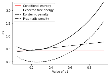
At \(\class{mj_yellow}{q=\left(\frac{1}{5},\frac{4}{5}\right)}\) the expected free energy dips just below the conditional entropy. What’s going on?
In short, the expected free energy is telling you to spend less time in unobserved state \(\class{mj_blue}{w_1}\) than you have been doing so far. That’s because being in \(\class{mj_blue}{w_1}\) only gives you a \(\frac{20}{25}=\frac{4}{5}\) chance of observing \(\class{mj_red}{x_2}\), and you want to observe \(\class{mj_red}{x_2}\) nine-tenths of the time. In contrast, if you were in state \(\class{mj_blue}{w_2}\) you would have a \(\frac{70}{75}=\frac{14}{15}\) chance of observing \(\class{mj_red}{x_2}\), which is much closer to the preferred distribution of \(\frac{9}{10}\).
Of course, by improving this pragmatic goal you suffer on the epistemic side of things: observing \(\class{mj_red}{x}\) no longer provides as much information about \(\class{mj_blue}{w}\). But this penalty increase is not great enough to counteract the penalty decrease you enjoy by better satisfying your goals regarding \(\class{mj_red}{x}\).