The active inference framework, spearheaded by Karl Friston and more commonly known in terms of its famous tenet, the free energy principle, has a reputation for being mathematically complex.
This is true.
If you have struggled with the concepts and calculations of active inference, you are not to blame.

And you are not alone. This short post is a first step to understanding Friston’s framework. I introduce the central concept of the framework – what it means to minimise free energy – for readers with minimal mathematical experience: all you’ll need to know is basic probability theory.
Everything is worked out explicitly, including calculations of free energy. There are diagrams to aid comprehension. The point is not to support or endorse active inference but to enable you to understand it.
(NB To be precise, this post describes variational inference, which is one of several techniques referred to by proponents of the active inference framework. To shield you from too much new terminology, I will just refer to minimising free energy in the rest of the post. You can understand the link between them as follows: variational inference is an activity that is achieved by minimising free energy.)
Model setup: where’s my cat?
You have a cat that spends its time in either the \(\class{mj_blue}{\text{kitchen}}\) or the \(\class{mj_blue}{\text{bedroom}}\). When it’s in the kitchen, it often \(\class{mj_red}{\text{meows}}\) for food; when it’s in the bedroom, it often \(\class{mj_red}{\text{purrs}}\) loudly.
Suppose you tally the proportion of the times your cat is in each place and making each noise. The results might look something like this:
$$ \begin{equation*} \begin{array}{cc} & & \class{mj_red}{\text{Cat noise}}\\ & & \begin{array}{cc} \class{mj_red}{\text{meow}} & \ \class{mj_red}{\text{purr}} \end{array}\\ \class{mj_blue}{\text{Cat location}}& \begin{array}{c} \class{mj_blue}{\text{kitchen}}\\ \class{mj_blue}{\text{bedroom}}\end{array} & \left(\begin{array}{c|c} 40\% & 20\%\\ \hline 10\% & 30\% \end{array}\right) \end{array} \end{equation*} $$
You can see that 40% of the time the cat is in the \(\class{mj_blue}{\text{kitchen}}\) and \(\class{mj_red}{\text{meowing}}\), and 30% of the time it is in the \(\class{mj_blue}{\text{bedroom}}\) and \(\class{mj_red}{\text{purring}}\). It does sometimes mix and match those locations and noises – sometimes it \(\class{mj_red}{\text{purrs}}\) in the \(\class{mj_blue}{\text{kitchen}}\) or \(\class{mj_red}{\text{meows}}\) in the \(\class{mj_blue}{\text{bedroom}}\) – but less frequently.
(NB: We are assuming that the cat cannot be anywhere but the \(\class{mj_blue}{\text{kitchen}}\) or the \(\class{mj_blue}{\text{bedroom}}\), and that it cannot make sounds other than \(\class{mj_red}{\text{meowing}}\) or \(\class{mj_red}{\text{purring}}\).)
Now suppose you are in the living room and you hear a \(\class{mj_red}{\text{meow}}\). You can’t tell whether the sound came from the \(\class{mj_blue}{\text{kitchen}}\) or \(\class{mj_blue}{\text{bedroom}}\), but you do know the statistics given in the table above. The free energy principle gives a way to answer the question: what is the probability of the cat being in one location or the other, given that we heard it \(\class{mj_red}{\text{meowing}}\)?
A simple solution: Basic probability theory
This model is so simple that we can answer our question with nothing more than basic probability theory. Let’s do that first, before moving onto the more complicated method involving free energy.
We want to know the probability of the cat being in each location, given that we heard it \(\class{mj_red}{\text{meowing}}\). So we really want two things: the probability of the cat being in the \(\class{mj_blue}{\text{kitchen}}\) given that we heard it \(\class{mj_red}{\text{meowing}}\), and the probability of it being in the \(\class{mj_blue}{\text{bedroom}}\) given that we heard it \(\class{mj_red}{\text{meowing}}\). Mathematically we write these as: $$ \begin{align} p(\class{mj_blue}{\text{kitchen}}&|\class{mj_red}{\text{meowing}})\\[0.8em] p(\class{mj_blue}{\text{bedroom}}&|\class{mj_red}{\text{meowing}}) \end{align} $$
These are conditional probabilities.
There is a very simple way to find these values. We can use the formula: $$ \begin{equation} p(\class{mj_blue}{w}|\class{mj_red}{x}) = \frac{p(\class{mj_blue}{w},\class{mj_red}{x})}{p(\class{mj_red}{x})} \end{equation} $$
The value on top of the fraction, \(p(\class{mj_blue}{w},\class{mj_red}{x})\), is called the joint probability. We have already encountered it: it’s just the percentages listed in the table above, converted into fractions: $$ \begin{alignat}{2} &p(\class{mj_blue}{\text{kitchen}},\class{mj_red}{\text{meowing}}) &&= \frac{4}{10}\\[0.8em] &p(\class{mj_blue}{\text{kitchen}},\class{mj_red}{\text{purring}}) &&= \frac{2}{10}\\[0.8em] &p(\class{mj_blue}{\text{bedroom}},\class{mj_red}{\text{meowing}}) &&= \frac{1}{10}\\[0.8em] &p(\class{mj_blue}{\text{bedroom}},\class{mj_red}{\text{purring}}) &&= \frac{3}{10} \end{alignat} $$
The value on the bottom of the fraction, \(p(\class{mj_red}{x})\), is called the marginal probability of \(\class{mj_red}{x}\). It is the overall probability that the cat is \(\class{mj_red}{\text{purring}}\) or \(\class{mj_red}{\text{meowing}}\). We can find it by summing the relevant joint probabilities:
$$ \begin{align} p(\class{mj_red}{\text{meowing}})& = \frac{4}{10} + \frac{1}{10}\\[0.8em] &= \frac{5}{10}\\[0.8em] p(\class{mj_red}{\text{purring}})& = \frac{2}{10} + \frac{3}{10}\\[0.8em] &= \frac{5}{10} \end{align} $$
Answering our question is as simple as plugging those numbers into the formula: $$ \begin{align} p(\class{mj_blue}{\text{kitchen}}|\class{mj_red}{\text{meowing}}) &= \frac{p(\class{mj_blue}{\text{kitchen}},\class{mj_red}{\text{meowing}})} {p(\class{mj_red}{\text{meowing}})}\\[0.8em] &= \frac{\frac{4}{10}}{\frac{5}{10}} = \frac{4}{5}\\[0.8em] p(\class{mj_blue}{\text{bedroom}}|\class{mj_red}{\text{meowing}}) &= \frac{p(\class{mj_blue}{\text{bedroom}},\class{mj_red}{\text{meowing}})} {p(\class{mj_red}{\text{meowing}})}\\[0.8em] &= \frac{\frac{1}{10}}{\frac{5}{10}} = \frac{1}{5} \end{align} $$
So when we hear the cat \(\class{mj_red}{\text{meowing}}\), we should conclude that the probability it is in the \(\class{mj_blue}{\text{kitchen}}\) is \(\frac{4}{5}\), and the probability that it is in the \(\class{mj_blue}{\text{bedroom}}\) is \(\frac{1}{5}\).
(NB I’m using the symbol \(\class{mj_blue}{w}\) to represent an unobserved state of the \(\class{mj_blue}{w}\text{orld,}\) and \(\class{mj_red}{x}\) to represent observed data. You can remember this because data are often caused by unobserved states, just as \(\class{mj_red}{x}\) comes right after \(\class{mj_blue}{w}\) in the alphabet. Some authors use \(s\) for the unobserved \(s\text{tate,}\) and \(o\) for the \(o\text{bserved data.}\))
The simple solution entails a simple principle
To prepare ourselves for the more complicated way of solving this problem, we need to introduce one more piece of terminology.
Suppose we are keeping track in our head of the probability of the location of the cat. This probability will change throughout the day as we hear different sounds. We will say that \(q(\class{mj_blue}{w})\) is our current estimate of where the cat is.
\(q(\class{mj_blue}{w})\) is a probability vector. It must contain two values that add up to 1. For example: $$ q(\class{mj_blue}{w})=\left(\frac{1}{2},\ \frac{1}{2}\right) $$
which means you are assigning a 50/50 chance to the cat being in the \(\class{mj_blue}{\text{kitchen}}\) or the \(\class{mj_blue}{\text{bedroom}}\). Or: $$ q(\class{mj_blue}{w})=\left(1,\ 0\right) $$
which means you are absolutely certain that the cat is in the \(\class{mj_blue}{\text{kitchen}}\), or: $$ q(\class{mj_blue}{w})=\left(0,\ 1\right) $$
which means you are absolutely certain that the cat is in the \(\class{mj_blue}{\text{bedroom}}\).
The problem posed above now becomes: what should the values of \(q(\class{mj_blue}{w})\) be given that we heard the cat \(\class{mj_red}{\text{meowing}}\)? Our simple answer was: $$ \begin{alignat}{2} q(&\class{mj_blue}{\text{kitchen}}) &&\leftarrow p(\class{mj_blue}{\text{kitchen}}|\class{mj_red}{\text{meowing}})\\[0.8em] q(&\class{mj_blue}{\text{bedroom}}) &&\leftarrow p(\class{mj_blue}{\text{bedroom}}|\class{mj_red}{\text{meowing}}) \end{alignat} $$
where the right hand side is calculated using the basic probability formula, as described above. The left-pointing arrow \(\leftarrow\) means, “set the value of the thing on the left to the value of the thing on the right.”
Call this the simple principle: it tells us that if we hear a \(\class{mj_red}{\text{meow}}\) we should choose the values of \(q(\class{mj_blue}{w})\) so that they are equal to \(p(\class{mj_blue}{w}|\class{mj_red}{\text{meow}})\).
It is worth pointing out that there is a correct answer to the question, what should \(q(\class{mj_blue}{w})\) be before the cat makes a noise? In this case, you simply count up the percentages in the table \(p(\class{mj_blue}{w},\class{mj_red}{x})\) for which the cat is in the \(\class{mj_blue}{\text{kitchen}}\) \(\left(40\%+20\%=60\%\right)\) versus the \(\class{mj_blue}{\text{bedroom}}\) \(\left(10\%+30\%=40\%\right)\). The result is the marginal probability of \(\class{mj_blue}{w}\), which is \(p(\class{mj_blue}{w})=\left(\frac{6}{10},\ \frac{4}{10}\right).\) The simple principle tells us that before hearing any noise we should choose the values of \(q(\class{mj_blue}{w})\) so that they are equal to \(p(\class{mj_blue}{w}).\)
A complex solution: minimising free energy
This model is so simple that using the free energy principle to solve it will be like using a sledgehammer to crack a nut. But practising with the sledgehammer will stand us in good stead to attack more complicated nuts.
The simple principle said: upon hearing \(\class{mj_red}{\text{meow}}\text{,}\) choose the values of \(q(\class{mj_blue}{w})\) so that they are equal to the conditional probabilities \(p(\class{mj_blue}{w}|\class{mj_red}{\text{meow}})\). We can write this as: $$ \begin{align} q(\class{mj_blue}{w})\leftarrow p(\class{mj_blue}{w}|\class{mj_red}{\text{meow}}) \end{align} $$
The free energy principle says: upon hearing \(\class{mj_red}{\text{meow}}\text{,}\) choose the values of \(q(\class{mj_blue}{w})\) so that a quantity called free energy, which we will cover in a moment, is as small as possible. We can write this as: $$ q(\class{mj_blue}{w})\leftarrow \underset{q(\class{mj_blue}{w})}{\operatorname{argmin}} F(p,q,\class{mj_red}{\text{meow}}) $$
The right-hand side of this statement has two parts.
The first part, \(\underset{q(\class{mj_blue}{w})}{\operatorname{argmin}}\), means “the value of \(q(\class{mj_blue}{w})\) such that the following term is as small as possible”.
The second part, \(F\), is a mathematical function called free energy. It takes as inputs the statistics \(p(\class{mj_blue}{w},\class{mj_red}{x})\), your beliefs \(q(\class{mj_blue}{w})\), and what you observe \(\class{mj_red}{\text{meow}}\). We will unpack free energy in more detail below.
For now, all you need to realise is that the free energy principle is doing the same kind of thing as the simple principle: it is telling you how to set the value of \(q(\class{mj_blue}{w})\) on the basis of something you’ve observed, namely \(\class{mj_red}{\text{meow}}\), and the statistical relationship \(p(\class{mj_blue}{w},\class{mj_red}{x})\).
The big difference is that the free energy principle isn’t telling you to choose \(q(\class{mj_blue}{w})\) so that it is equal to something. It is telling you to choose \(q(\class{mj_blue}{w})\) so that free energy, whose value depends on \(q(\class{mj_blue}{w})\), is as small as possible. An analogy will make this clearer.
An analogy: the fenced enclosure principle
Suppose you are given a length of fencing with which to enclose an area of ground. The “fenced enclosure principle” says: choose the shape of fencing that encloses the largest area. If we say that \(s\) stands for the shape of the fencing you lay out, and \(A\) is the area enclosed by that shape, we can write the fenced enclosure principle as: $$ s \leftarrow \underset{s}{\operatorname{argmax}} A(s) $$
This says: choose the shape \(s\) such that the area \(A\) is as large as possible. (The fenced enclosure principle uses “argmax” instead of “argmin”, because you want the largest enclosure.)
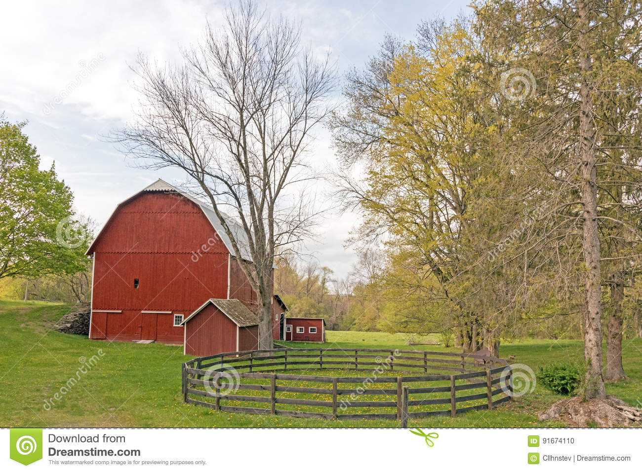
You can try lots of different ways of fencing off areas and measuring them…
…until you find the arrangement producing the largest possible area: a circle.
The different possible arrangements \(s\) are analogous to different belief vectors \(q(\class{mj_blue}{w})\). The different sizes of fenced enclosure \(A\) are analogous to different values of free energy \(F\).
So what is free energy?
The actual definition of free energy looks a bit scary: $$ F= \class{mj_green}{\sum_{\class{mj_blue}{w}} \left( q(\class{mj_blue}{w}) \class{mj_lavender}{\log \left( \frac{q(\class{mj_blue}{w})} {p(\class{mj_blue}{w},\class{mj_red}{x})} \right)} \right)} $$
If your eyes have glazed over, I totally understand. Stick with me.
Forget for a moment about the justification for using this term to guide inference. Just notice a few things about the definition. First, it contains two terms we’ve already met: \(p(\class{mj_blue}{w},\class{mj_red}{x})\) and \(q(\class{mj_blue}{w})\). There are a couple of unfamiliar terms though, \(\class{mj_green}{\sum_{\class{mj_blue}{w}}}\) and \(\class{mj_lavender}{\log{}}\). Fortunately they are easy to understand:
- \(\class{mj_green}{\sum_{\class{mj_blue}{w}}\left(\right)}\) says: gather all the possible states of \(\class{mj_blue}{w}\) and insert them into the term in brackets one by one. You will end up with a bunch of different values, one for each possible state of \(\class{mj_blue}{w}\). Add all these values together. Example: suppose that \(\class{mj_orange}{a}\) is the set of values \(\class{mj_orange}{\{1,2,3\}}\), then \(\class{mj_green}{\sum_{\class{mj_orange}{a}}\left(\class{mj_orange}{a}\right)}=\class{mj_orange}{1}+\class{mj_orange}{2}+\class{mj_orange}{3}=6\), and \(\class{mj_green}{\sum_{\class{mj_orange}{a}}\left(\frac{\class{mj_orange}{a}}{2}\right)}=\frac{\class{mj_orange}{1}}{2}+\frac{\class{mj_orange}{2}}{2}+\frac{\class{mj_orange}{3}}{2}=3\). The symbol that looks like a funky capital E is the Greek capital letter Sigma, and is very often used to indicate this kind of summation.
- \(\class{mj_lavender}{\log{\left(\right)}}\) says: take the logarithm of the term in brackets. A logarithm is just a function that turns one number into another. When the term in brackets is a ratio, as it is here, the logarithm is often used to compare the two. (You can see this thanks to a useful mathematical fact: \(\class{mj_lavender}{\log{\frac{q}{p}}}=\class{mj_lavender}{\log{q}}-\class{mj_lavender}{\log{p}}.\) In other words, a logarithm of a ratio is really just a difference, and differences tell you how far apart two things are.) Very roughly, you can think about it this way: \(q(\class{mj_blue}{w})\) is your belief about the probabilities, and \(p(\class{mj_blue}{w},\class{mj_red}{x})\) encapsulates the “correct” probabilities, so taking the logarithm of their ratio is a way of determining how accurate your beliefs are. This isn’t exactly right, but it’s worth understanding things in this not-quite-right way just to get a handle on the concepts.
Altogether, with defined values for \(p(\class{mj_blue}{w},\class{mj_red}{x})\), \(q(\class{mj_blue}{w})\) and \(\class{mj_red}{x}\), the function \(F\) will yield a specific value. Below, we will calculate \(F\) for various values of \(q(\class{mj_blue}{w})\) and \(\class{mj_red}{x}\).
Solving the problem by minimising free energy
We have the joint distribution \(p(\class{mj_blue}{w},\class{mj_red}{x})\) representing the statistical connection between our cat’s location and the noises it makes. We hear a \(\class{mj_red}{\text{meow}}\), which determines our value of \(\class{mj_red}{x}=\class{mj_red}{\text{meow}}\). What should \(q(\class{mj_blue}{w})\) be? How confident should we be that our cat is in the \(\class{mj_blue}{\text{kitchen}}\) or the \(\class{mj_blue}{\text{bedroom}}\)?
The free energy principle says that \(q(\class{mj_blue}{w})\) should be the vector that makes \(F\) as small as possible: $$ q(\class{mj_blue}{w})\leftarrow \underset{q(\class{mj_blue}{w})}{\operatorname{argmin}} F(p,q,\class{mj_red}{\text{meow}}) $$
We already have values for \(p(\class{mj_blue}{w},\class{mj_red}{x})\) and \(\class{mj_red}{x}\), so we can test a bunch of different values of \(q(\class{mj_blue}{w})\) and see which one makes \(F\) smallest – exactly like trying a bunch of different fencing shapes and seeing which one makes the enclosed area largest.
The good news is that we can draw a graph of \(F\). This will help us understand what’s going on. Because \(\class{mj_blue}{w}\) only has two values, \(\class{mj_blue}{\text{kitchen}}\) and \(\class{mj_blue}{\text{bedroom}}\), once you’ve chosen the first entry in \(q(\class{mj_blue}{w})\) the second entry is determined for you. This means we can graph it: we will let the x-axis represent the first entry in \(q(\class{mj_blue}{w})\), and the y-axis represent free energy \(F\).
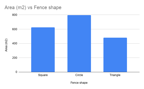
Let’s see what happens when we consider four possible values for \(q(\class{mj_blue}{\text{kitchen}})\):
What is this graph telling us? It says: of these four options, the one with the lowest free energy is \(q(\class{mj_blue}{\text{kitchen}})=\frac{4}{5}\). Just as we picked the fence shape that yielded the largest enclosed area, we should pick the degree of belief that yields the lowest free energy.
But what if we allow our degree of belief to range over every possible value between \(0\) and \(1\)? The result is as follows:
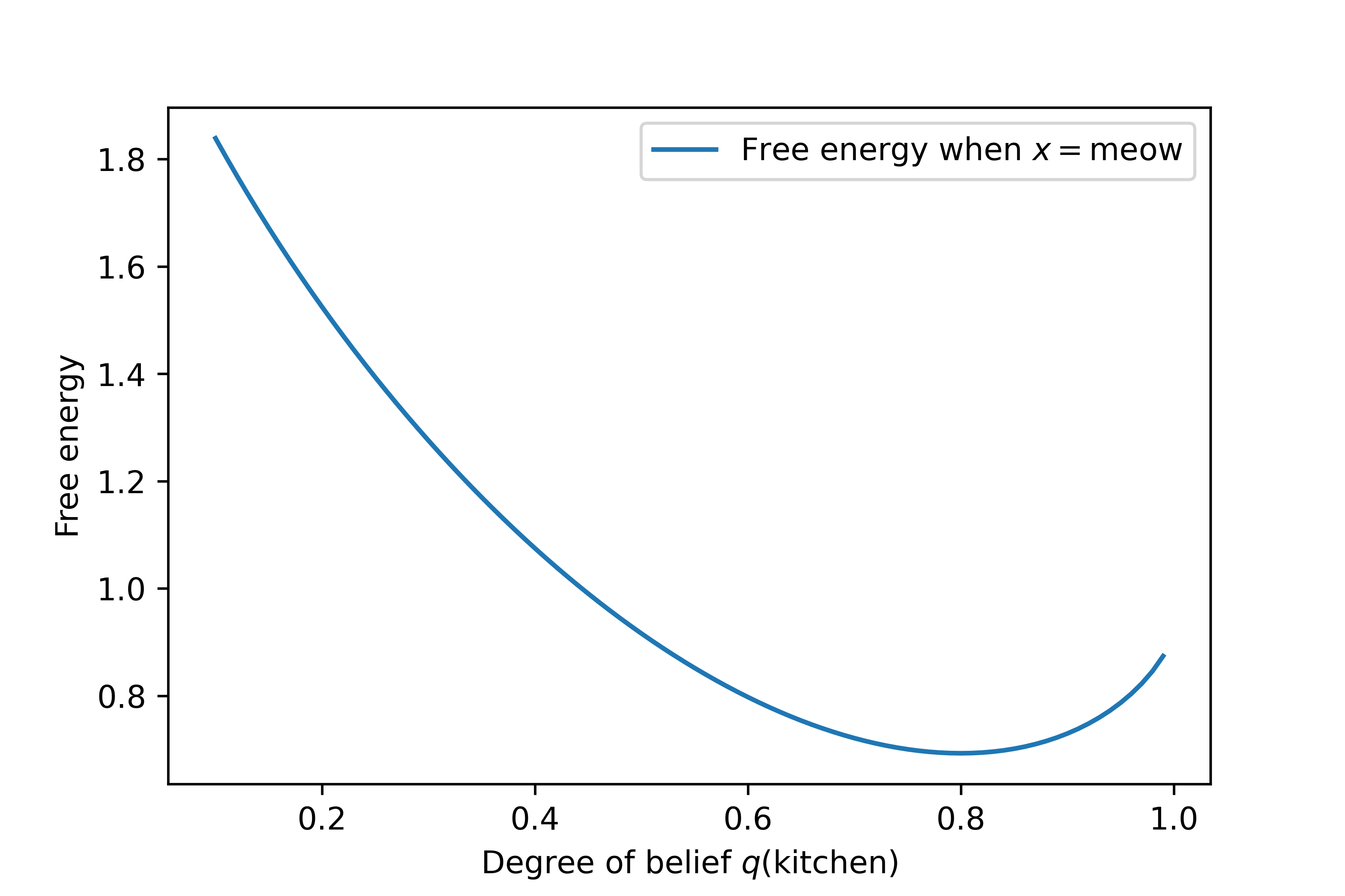
It still looks like the smallest possible value of \(F\) occurs when the value of \(q(\class{mj_blue}{\text{kitchen}})\) is 0.8; that is, when our degree of belief that the cat is in the kitchen is about \(\frac{4}{5}\). And since our value for \(q(\class{mj_blue}{\text{kitchen}})\) determines our value for \(q(\class{mj_blue}{\text{bedroom}})\), our degree of belief that the cat is in the bedroom must be \(q(\class{mj_blue}{\text{bedroom}})=\frac{1}{5}\).
As a result, the free energy principle tells us that our solution to the problem should be: $$ q(\class{mj_blue}{w}) = \left(\frac{4}{5},\frac{1}{5}\right) \quad\quad \text{if \(\class{mj_red}{x}=\class{mj_red}{\text{meow}}\)} $$
This is the same solution we found by following the simple principle.
For completeness, here is the equivalent graph when \(\class{mj_red}{x}=\class{mj_red}{\text{purr}}\):
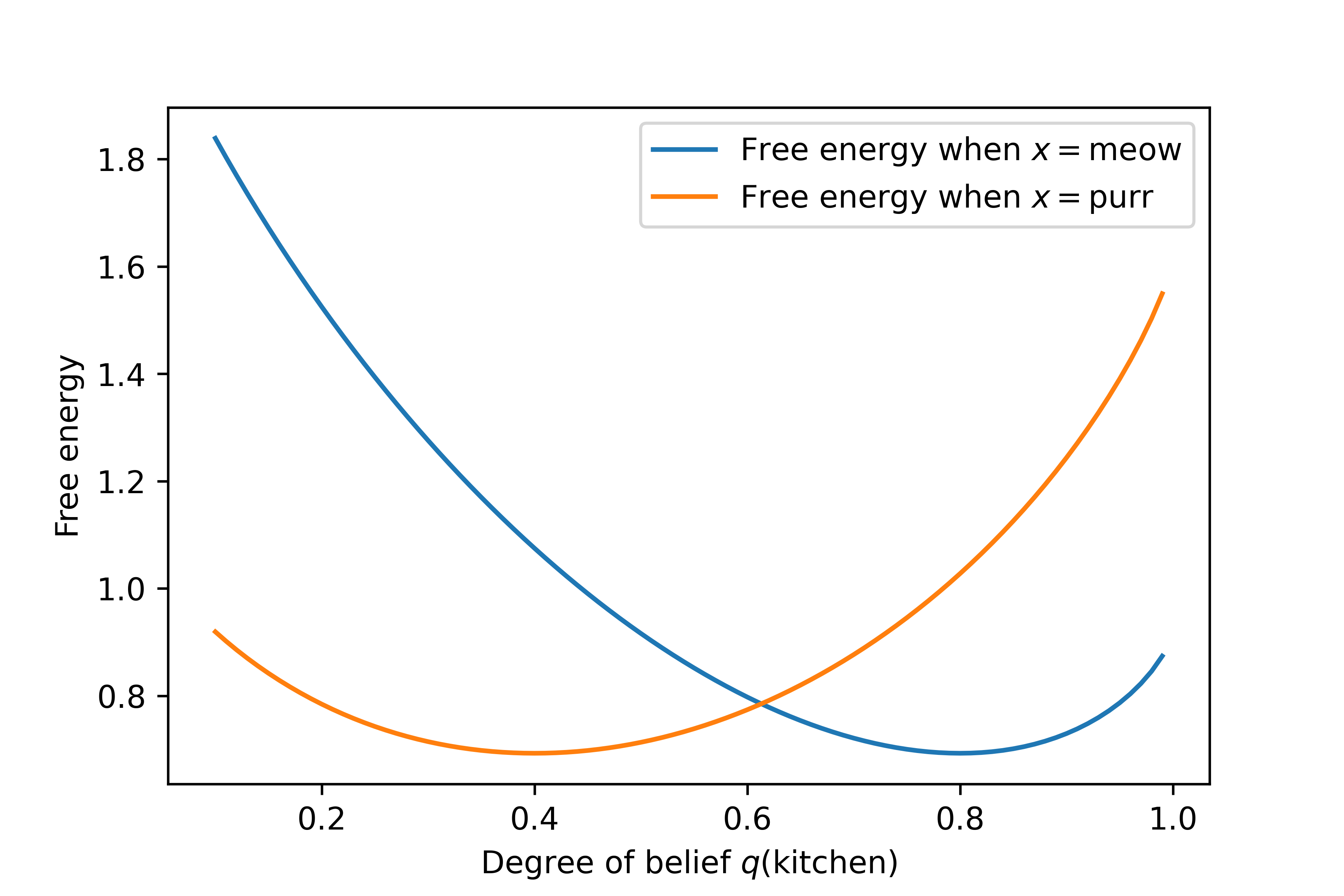
Now the smallest value of \(F\) occurs when \(q(\class{mj_blue}{\text{kitchen}})=0.4\), which is \(\frac{2}{5}\). The full answer to the problem in this case is: $$ q(\class{mj_blue}{w}) = \left(\frac{2}{5},\frac{3}{5}\right) \quad\quad \text{if \(\class{mj_red}{x}=\class{mj_red}{\text{purr}}\)} $$
If you go back and follow the simple principle, inserting \(\class{mj_red}{x}=\class{mj_red}{\text{purr}}\) and calculating the conditional probabilities, you will reach the same result.
How the sledgehammer earns its keep
“Hang on a minute” some of you are probably thinking. “If the free energy principle gives the same answer as the simple principle, surely we should be using the simpler of the two.”
You’re half right: problems as simple as this one can be solved using basic probability theory. At this stage, all we have shown is that this fancy free-energy stuff is consistent with the simple principle, which is kind of a minimum requirement.
But you’re also half wrong: problems more complex than this cannot usually be solved using basic probability theory. When you look further, you will find situations where minimising free energy is the only available solution. Why might that be?
Recall how we followed the simple principle by calculating the conditional probability: $$ q(\class{mj_blue}{w}) \leftarrow p(\class{mj_blue}{w}|\class{mj_red}{x}) = \frac{p(\class{mj_blue}{w},\class{mj_red}{x})}{p(\class{mj_red}{x})} $$
The free energy principle comes in handy when this formula cannot be used. Crucially, \(p(\class{mj_red}{x})\) is sometimes impossible to calculate. In particular, when we move beyond discrete probability distributions (i.e. those that have distinct states like \(\class{mj_red}{\text{meow}}, \class{mj_red}{\text{purr}}\) and so on), many continuous probability distributions are so unwieldy that finding \(p(\class{mj_red}{x})\) is an intractable problem.
In these circumstances, the best you can do is approximate the simple principle. Minimising free energy is one well-understood way of doing so.
Explaining the relationship between the two principles – why minimising \(F\) is a good approximation to finding \(p(\class{mj_blue}{w}|\class{mj_red}{x})\), and why \(p(\class{mj_red}{x})\) is sometimes impossible to calculate – is beyond the scope of this post. I hope, however, you now grasp the basic sense of the free energy principle, and are in a better position to approach those more difficult themes.